Histograms and Frequency Distributions

To demonstrate the construction of histograms and frequency distributions we will use the data in the example below.

Example: The table below lists the number of medals won by country in the 2012 Summer Olympics.

Country	Number of Medals
United States	104
China	88
Russia	82
Great Britain	65
Germany	44
Japan	38
Australia	35
France	34
South Korea	28
Italy	28
Netherlands	20
Ukraine	20
Canada	18
Hungary	17
Spain	17
Cuba	14
Kazakhstan	13
New Zealand	13
Iran	12
Jamaica	12

Source: wikipedia.org

First we'll need to create a data set.

> medals = c(104, 88, 82, 65, 44, 38, 35, 34, 28, 28, 20, 20, 18, 17, 17, 14, 13, 13, 12, 12)

Creating a Histogram

Histograms can be quickly created with the hist command.

> hist(medals)

This command generates a histogram from our data, but chooses its own class width.  In order to change the number of classes we can include the breaks argument.  For instance, instead of the 6 classes R created by default, let's create another histogram from this data with 10 classes.

> hist(medals, breaks = 10)

By setting breaks = 10 we now have a histogram with 10 classes.  Unfortunately, using the breaks argument in this fashion is only a suggestion.  If we repeat this command with breaks = 12 we will end up with the same graph, and still only 10 classes.

What we need, then, is a way to ensure this command gives us exactly the number of classes we want, along with the appropriate lower and upper class boundaries.  To start, let's find the minimum and maximum values in our data set.

> min(medals)
[1] 12
> max(medals)
[1] 104

Since our data values range from 12 to 104 we can choose to construct a histogram that ranges from 10 to 110, with a class width of 5.  In order to require R to follow these specific guidelines we will use the seq command to make our breaks a sequence of values from 5 to 110, counting by 5's.

> hist(medals, breaks = seq(10, 110, 5))

We could also choose a class width of 2, 10, 20, or any value that can be equally distributed across the range of values for our histogram.

If we want to add more information to our plot we can include the main and xlab arguments.

> hist(medals, breaks = seq(10, 110, 5), main = "Histogram of Medals Won", xlab = "Number of Medals")

Creating a Frequency Distribution

There is no simple command to create a frequency distribution in R, but we can output the numerical information from the graph by including the argument plot = FALSE.

> hist(medals, breaks = seq(10, 110, 5), plot = FALSE)
$breaks
 [1]  10  15  20  25  30  35  40  45  50  55  60  65  70  75  80  85  90  95 100
[20] 105 110

$counts
 [1] 5 5 0 2 2 1 1 0 0 0 1 0 0 0 1 1 0 0 1 0

$intensities
 [1] 0.05 0.05 0.00 0.02 0.02 0.01 0.01 0.00 0.00 0.00 0.01 0.00 0.00 0.00 0.01
[16] 0.01 0.00 0.00 0.01 0.00

$density
 [1] 0.05 0.05 0.00 0.02 0.02 0.01 0.01 0.00 0.00 0.00 0.01 0.00 0.00 0.00 0.01
[16] 0.01 0.00 0.00 0.01 0.00

$mids
 [1]  12.5  17.5  22.5  27.5  32.5  37.5  42.5  47.5  52.5  57.5  62.5  67.5
[13]  72.5  77.5  82.5  87.5  92.5  97.5 102.5 107.5

$xname
[1] "medals"

$equidist
[1] TRUE

attr(,"class")
[1] "histogram"

From this information we can pull out the right and left endpoints for each class ($breaks), and the frequency of each class ($counts) to create the frequency distribution below.

Class	Frequency
(10-15]	5
(15-20]	5
(20-25]	0
(25-30]	2
(30-35]	2
(35-40]	1
(40-45]	1
(45-50]	0
(50-55]	0
(55-60]	0
(60-65]	1
(65-70]	0
(70-75]	0
(75-80]	0
(80-85]	1
(85-90]	1
(90-95]	0
(95-100]	0
(100-105]	1
(105-110]	0

Left-Closed (Right Open) Intervals

By default, R constructs histograms with class intervals that are right-closed (left open).  If instead we wanted class intervals that are left-closed (right open), we can include the argument right = FALSE.

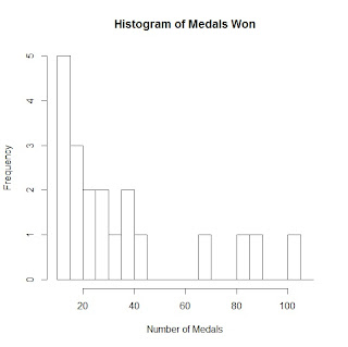
> hist(medals, breaks = seq(10, 110, 5), right = FALSE, main = "Histogram of Medals Won", xlab = "Number of Medals")

> hist(medals, breaks = seq(10, 110, 5), right = FALSE, plot = FALSE)
$breaks
 [1]  10  15  20  25  30  35  40  45  50  55  60  65  70  75  80  85  90  95 100
[20] 105 110

$counts
 [1] 5 3 2 2 1 2 1 0 0 0 0 1 0 0 1 1 0 0 1 0

$intensities
 [1] 0.05 0.03 0.02 0.02 0.01 0.02 0.01 0.00 0.00 0.00 0.00 0.01 0.00 0.00 0.01
[16] 0.01 0.00 0.00 0.01 0.00

$density
 [1] 0.05 0.03 0.02 0.02 0.01 0.02 0.01 0.00 0.00 0.00 0.00 0.01 0.00 0.00 0.01
[16] 0.01 0.00 0.00 0.01 0.00

$mids
 [1]  12.5  17.5  22.5  27.5  32.5  37.5  42.5  47.5  52.5  57.5  62.5  67.5
[13]  72.5  77.5  82.5  87.5  92.5  97.5 102.5 107.5

$xname
[1] "medals"

$equidist
[1] TRUE

attr(,"class")
[1] "histogram"